1. Overview & Download
Many molecular high-throughput experiments result in high-dimensional data matrices with the number of features (represented in the rows) being much larger than the number of samples (represented in the columns). Since multiple features are measured on the same experimental unit, the data can be regarded as repeated measurements.
The R-package 'RepeatedHighDim' comprises a selection of functions for different aspects of the analysis of high-dimensional repeated measurements. In particular, functions for
- outlier detection,
- differential expression analysis,
- network meta-analysis of gene expression studies
- self contained gene-set tests,
- and the generation of binary random data
are provided.
This documentation details the functionality of the package and guides through the example code. In the code examples, input is printed in red, output is printed in blue color.
Download is available from The Comprehensive R Archive Network.
2. Outlier detection
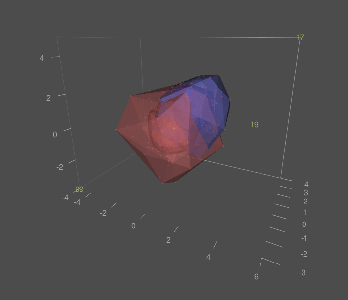
A first step in exploratory data analysis of high-dimensional data is unsupervised clustering of samples in a lower-dimensional space, for example by means of principal component analysis (PCA). This analysis step can also be used to detect outlying samples. RepeatedHighDim implements the graphical approach of gemplots in the space of the first three principal components (Kruppa & Jung, 2017). This method extends the idea of bagplots, the two-dimensional version of boxplots (Rousseeuw et al., 1999). The advantage of the presented approach is that the data of multiple groups can be represented in the same PCA plot, but outlier detection is performed separately for each group.
As an example, consider data 400 experimental units from two experimental groups in a three-dimensional space:
## Two 3-dimensional example data sets D1 and D2
n <- 200
x1 <- rnorm(n, 0, 1)
y1 <- rnorm(n, 0, 1)
z1 <- rnorm(n, 0, 1)
D1 <- data.frame(cbind(x1, y1, z1))
x2 <- rnorm(n, 1, 1)
y2 <- rnorm(n, 1, 1)
z2 <- rnorm(n, 1, 1)
D2 <- data.frame(cbind(x2, y2, z2))
colnames(D1) <- c("x", "y", "z")
colnames(D2) <- c("x", "y", "z")
|
Next, we replace one observation in each group by an outlier:
## Placing outliers in D1 and D2
D1[17,] = c(4, 5, 6)
D2[99,] = -c(3, 4, 5)
|
Before the gemplots can be calculated and visualized, some graphical parameters need to be specified:
## Grid size and graphic parameters
grid.size <- 20
red <- rgb(200, 100, 100, alpha = 100, maxColorValue = 255)
blue <- rgb(100, 100, 200, alpha = 100, maxColorValue = 255)
yel <- rgb(255, 255, 102, alpha = 100, maxColorValue = 255)
white <- rgb(255, 255, 255, alpha = 100, maxColorValue = 255)
require(rgl)
material3d(color=c(red, blue, yel, white), alpha=c(0.5, 0.5, 0.5, 0.5), smooth=FALSE, specular="black")
|
Now, the inner and outer gems can be calculated and visualized in for both groups in an interactive rgl-window:
## Calucation and visualization of gemplot for D1
G <- gridfun(D1, grid.size=20)
G$H <- hldepth(D1, G, verbose=TRUE)
dm <- depmed(G)
B <- bag(D1, G)
L <- loop(D1, B, dm=dm)
rgl.open()
points3d(D1[L$outliers==0,1], D1[L$outliers==0,2], D1[L$outliers==0,3], col=red)
text3d(D1[L$outliers==1,1], D1[L$outliers==1,2], D1[L$outliers==1,3], as.character(which(L$outliers==1)), col=yel)
spheres3d(dm[1], dm[2], dm[3], col=yel, radius=0.1)
gem(B$coords, B$hull, red)
gem(L$coords.loop, L$hull.loop, red)
axes3d(col="white")
## Calucation and visualization of gemplot for D2
G <- gridfun(D2, grid.size=20)
G$H <- hldepth(D2, G, verbose=TRUE)
dm <- depmed(G)
B <- bag(D2, G)
L <- loop(D2, B, dm=dm)
points3d(D2[L$outliers==0,1], D2[L$outliers==0,2], D2[L$outliers==0,3], col=red)
text3d(D2[L$outliers==1,1], D2[L$outliers==1,2], D2[L$outliers==1,3], as.character(which(L$outliers==1)), col=yel)
spheres3d(dm[1], dm[2], dm[3], col=yel, radius=0.1)
gem(B$coords, B$hull, blue)
gem(L$coords.loop, L$hull.loop, blue)
|
The gemplots and the outliers are shown:
|
3. Differential expression analysis
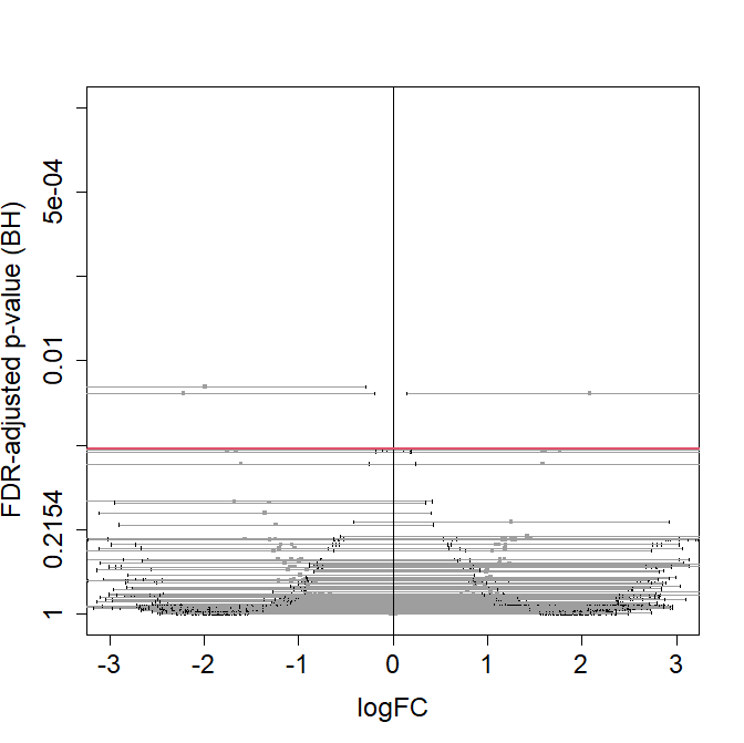
The effect measure typically used in differential expression analysis if the log fold change (logFC). While one part of analysts rely on p-values for the ranking and selection of genes, others rely on the logFC. However, while p-values incorporate informatin about variance and sample size, the logFC is only based on mean expression levels. Calculating confidence intervals for the logFC allows to use the logFC complementary to p-values (Jung et al., 2011). RepeatedHighDim provides functions to calculate confidence intervals given logFCs and their standard errors. Furthermore, confidence intervals can be FDR-adjusted complementary to the FDR-adjustment of p-values. Thus, logFCs with confidence intervals and p-values can lead to the same selections. The following example takes logFCs and their errors from the R-package limma.
### Artificial microarray data
d = 1000 ### Number of genes
n = 10 ### Sample per group
fc = rlnorm(d, 0, 0.1)
mu1 = rlnorm(d, 0, 1) ### Mean vector group 1
mu2 = mu1 * fc ### Mean vector group 2
sd1 = rnorm(d, 1, 0.2)
sd2 = rnorm(d, 1, 0.2)
X1 = matrix(NA, d, n) ### Expression levels group 1
X2 = matrix(NA, d, n) ### Expression levels group 2
for (i in 1:n) {
X1[,i] = rnorm(d, mu1, sd=sd1)
X2[,i] = rnorm(d, mu2, sd=sd2)
}
X = cbind(X1, X2)
### Differential expression analysis with limma
group = gl(2, n)
design = model.matrix(~ group)
fit1 = limma::lmFit(X, design)
fit = limma::eBayes(fit1)
### Calculation of confidence intervals
CI = fc_ci(fit=fit, alpha=0.05, method="raw")
#head(CI)
CI = fc_ci(fit=fit, alpha=0.05, method="BY")
#head(CI)
CI = fc_ci(fit=fit, alpha=0.05, method="BH")
head(CI)
p.bh logFC lower.bh upper.bh
1 0.9683291 0.1968580 -2.091356 2.485072
2 0.9047641 0.4168695 -1.808479 2.642218
3 0.9047641 0.4042321 -1.531589 2.340053
4 0.9582795 0.1680394 -1.570448 1.906527
5 0.8748515 -0.5192362 -2.416081 1.377608
6 0.7980203 -0.6557056 -2.389698 1.078287
### Visualization of confidence intervals and p-values in
### volcano plots.
#fc_plot(CI, xlim=c(-0.5, 3), ylim=-log10(c(1, 0.0001)), updown="up")
#fc_plot(CI, xlim=c(-3, 0.5), ylim=-log10(c(1, 0.0001)), updown="down")
fc_plot(CI, xlim=c(-3, 3), ylim=-log10(c(1, 0.0001)), updown="all")
|
Volcano plot with CIs for the logFC:
|
4. Network meta-analysis of gene expression studies
As thousands of public gene expression studies are available (e.g. from the gene expression omnibus or the array express databases) research synthesis in the form of meta-analyses or analyses of merged data sets is possible. Besides classical meta-analysis which aggregates information from studies that have the same design, network meta-analysis provides the possibility to build networks from studies of different designs. Group comparisons that have not been made in the original studies can than be conducted in the network meta-analysis. In RepeatedHighDim, a simple study network of gene expression studies can be analysed. Consider, one study involves a control group and a group with disease A. Another study involves a control group and a disease group B. If the control groups of the two studies are comparable, both studies can be linked via their control groups, and an indirect comparison between disease A and B is possible (Rücker, 2012). The function 'netRNA' take logFCs (between control and disease X) and their standard deviations from both studies as input and calculated the logFCs and their standard deviations between groups A and B (Winter et al., 2019).
#######################
### Data generation ###
#######################
n = 100 ### Sample size per group
G = 100 ### Number of genes
### Basic expression, fold change, batch effects and error
alpha.1 = rnorm(G, 0, 1)
alpha.2 = rnorm(G, 0, 1)
beta.1 = rnorm(G, 0, 1)
beta.2 = rnorm(G, 0, 1)
gamma.1 = rnorm(G, 0, 1)
gamma.2 = rnorm(G, 2, 1)
delta.1 = sqrt(invgamma::rinvgamma(G, 1, 1))
delta.2 = sqrt(invgamma::rinvgamma(G, 1, 2))
sigma.g = rep(1, G)
# Generate gene names
gene_names = paste("Gene", 1:G, sep = "")
### Data matrices of control and treatment (disease) groups
C.1 = matrix(NA, G, n)
C.2 = matrix(NA, G, n)
T.1 = matrix(NA, G, n)
T.2 = matrix(NA, G, n)
for (j in 1:n) {
C.1[,j] = alpha.1 + (0 * beta.1) + gamma.1 + (delta.1 * rnorm(1, 0, sigma.g))
C.2[,j] = alpha.1 + (0 * beta.2) + gamma.2 + (delta.2 * rnorm(1, 0, sigma.g))
T.1[,j] = alpha.2 + (1 * beta.1) + gamma.1 + (delta.1 * rnorm(1, 0, sigma.g))
T.2[,j] = alpha.2 + (1 * beta.2) + gamma.2 + (delta.2 * rnorm(1, 0, sigma.g))
}
study1 = cbind(C.1, T.1)
study2 = cbind(C.2, T.2)
# Assign gene names to row names
#rownames(study1) = gene_names
#rownames(study2) = gene_names
#############################
### Differential Analysis ###
#############################
if(check_limma()){
### study1: treatment A versus control
group = gl(2, n)
M = model.matrix(~ group)
fit = limma::lmFit(study1, M)
fit = limma::eBayes(fit)
p.S1 = fit$p.value[,2]
fc.S1 = fit$coefficients[,2]
fce.S1 = sqrt(fit$s2.post) * sqrt(fit$cov.coefficients[2,2])
### study2: treatment B versus control
group = gl(2, n)
M = model.matrix(~ group)
fit = limma::lmFit(study2, M)
fit = limma::eBayes(fit)
p.S2 = fit$p.value[,2]
fc.S2 = fit$coefficients[,2]
fce.S2 = sqrt(fit$s2.post) * sqrt(fit$cov.coefficients[2,2])
#############################
### Network meta-analysis ###
#############################
p.net = rep(NA, G)
fc.net = rep(NA, G)
treat1 = c("uninfected", "uninfected")
treat2 = c("ZIKA", "HSV1")
studlab = c("experiment1", "experiment2")
fc.true = beta.2 - beta.1
TEs = list(fc.S1, fc.S2)
seTEs = list(fce.S1, fce.S2)
}
# Example usage:
test = netRNA(TE = TEs, seTE = seTEs, treat1 = treat1, treat2 = treat2, studlab = studlab)
|
Finally, the output object 'test' contains a list which includes p-values, logFCs (between groups A and B) plus their 95%-confidence intervals for each gene.
5. Gene set analysis
Besides studying expression changes of individual genes, a typical step in transciptomics data analysis is to study effects of gene-sets. The most common type of gene-set analysis is enrichment analysis which relies on the results of differential expression analysis. The occurence of gene-set members among the top ranked genes is compared to the occurence of member among non-top ranked genes is compared. Hence, enrichment methods are sometimes referred to as 'competitive' gene-set tests'. In contrast, 'self-contained' gene-set tests directly compare the expression profile of the gene-set between different experimental groups (Jung et al., 2011).
Consider gene expression data of a subset of 100 genes from two experimental groups. The expression data of this subset can simply be committed the function RHighDim. In addition, the user needs to specify whether samples are paired or unpaired:
### Global comparison of a set of 100 genes between two experimental groups.
X1 = matrix(rnorm(1000, 0, 1), 10, 100)
X2 = matrix(rnorm(1000, 0.1, 1), 10, 100)
RHD = RHighDim(X1, X2, paired=FALSE)
|
The summary can be displayed as follows:
summary_RHD(RHD)
Number of Genes: 10
Number of Samples in Group 1: 100
Number of Samples in Group 2: 100
Samples are Paired: FALSE
effect F df1 df2 p
1 Group 1.2307 9.9801 1972.612 0.266
|
In the case that there are missing values, what sometimes occures in protein expression data (Jung et al., 2014), the function GlobTestMissing can be used which performs a permutation test. Here is an example with a subset of 100 proteins and 10 percent of missing values.
### Global comparison of a set of 100 proteins between two experimental groups,
### where (tau * 100) percent of expression levels are missing.
n1 = 10
n2 = 10
d = 100
tau = 0.1
X1 = t(matrix(rnorm(n1*d, 0, 1), n1, d))
X2 = t(matrix(rnorm(n2*d, 0.1, 1), n2, d))
X1[sample(1:(n1*d), tau * (n1*d))] = NA
X2[sample(1:(n2*d), tau * (n2*d))] = NA
GlobTestMissing(X1, X2, nperm=100)
Loading required package: nlme
$pval
[1] 0.02
|
6. Correlated binary data
Correlated binary variables regularly occur in biomedical research. In order to perform simulations with such data, methods for their artificial generation are necessary. This package provides functionality to sample a matrix of correlated binary data from specified distribution with given covariance matrix and marginal probabilities. The generation is based on a genetic algorithm, where a start matrix with specified marginal probabilities is modified until the specified correlation structure is approached (Kruppa et al., 2018).
In the following example a representative matrix with specified marginal probabilities and specified correlation matrix is generated. Then, a random sample is drawn from this matrix.
### Initialization of the start matrix with specified
### marginal probabilities p:
X0 <- start_matrix(p = c(0.5, 0.6), k = 10000)
table(X0[,1])
0 1
5000 5000
table(X0[,2])
0 1
4000 6000
### Generation of representative matrix Xt with specified
### marginal probabilities p and specified correlation matrix R
Xt <- iter_matrix(X0, R = diag(2), T = 10000, e.min = 0.00001)$Xt
[1] "10 %"
[1] "20 %"
[1] "30 %"
[1] "40 %"
table(Xt[,1])
0 1
5000 5000
table(Xt[,2])
0 1
4000 6000
cor(Xt)
[,1] [,2]
[1,] 1.00000000 0.07062695
[2,] 0.07062695 1.00000000
### Drawing of a random sample S of size n = 10
S <- Xt[sample(1:1000, 10, replace = TRUE),]
table(S[,1])
0 1
6 4
table(S[,2])
0 1
8 2
cor(S)
[,1] [,2]
[1,] 1.0000000 0.1020621
[2,] 0.1020621 1.0000000
|
Other contributors
Many thanks to
- Jochen Kruppa (University of Applied Sciences Osnabrück)
- Sergej Ruff (University of Veterinary Medicine Hannover)
for their contributions and their help to implement this package!
References
- Jung K, Becker B, Brunner B and Beissbarth T (2011). Comparison of Global Tests for Functional Gene Sets in Two-Group Designs and Selection of Potentially Effect-causing Genes. Bioinformatics, 27, 1377-1383.
[Open access]
- Jung K, Dihazi H, Bibi A, Dihazi GH and Beissbarth T (2014): Adaption of the Global Test Idea to Proteomics Data with Missing Values. Bioinformatics, 30, 1424-30.
[Open access]
- Jung K, Friede T and Beißbarth T (2011). Reporting FDR analogous confidence intervals for the log fold change of differentially expressed genes. BMC bioinformatics, 12, 1-9.
[Open access]
- Rücker G (2011). Network meta-analysis, electrical networks and graph theory. Research synthesis methods, 3(4), 312-324.
[Open access]
- Winter C, Kosch R, Ludlow M, Osterhaus AD, & Jung K (2019). Network meta-analysis correlates with analysis of merged independent transcriptome expression data. BMC bioinformatics, 20, 1-10.
[Open access]
- Kruppa, J., & Jung, K. (2017). Automated multigroup outlier identification in molecular high-throughput data using bagplots and gemplots. BMC bioinformatics, 18(1), 1-10.
[Open access]
- Kruppa, J., Lepenies, B., & Jung, K. (2018). A genetic algorithm for simulating correlated binary data from biomedical research. Computers in biology and medicine, 92, 1-8.
[Abstract]
- Rousseeuw, P. J., Ruts, I., & Tukey, J. W. (1999). The bagplot: a bivariate boxplot. The American Statistician, 53(4), 382-387.
[Abstract]
Contact
Prof. Dr. Klaus Jung
University of Veterinary Medicine Hannover, Foundation
Institute for Animal Breeding and Genetics
Bünteweg 17p, D-30559 Hannover, Germany
klaus.jung@tiho-hannover.de
www.klausjung-lab.de |